Videos
The variation of the gyrokinetic drift velocity along the unperturbed field lines
The gyro-averaged drift velocity for (left) electrons and (right) ions is shown as it varies along the unperturbed field lines (z direction). The effect of the strong gyro-average is observed for the ions. The animations are done for a single point in velocity phase space.
[Diagnostics and animations by Evgeny Gorbunov 2020, using numerical simulations performed by Dr. Daniel Told with the GENE code.]
Looping gif version: ions | electrons
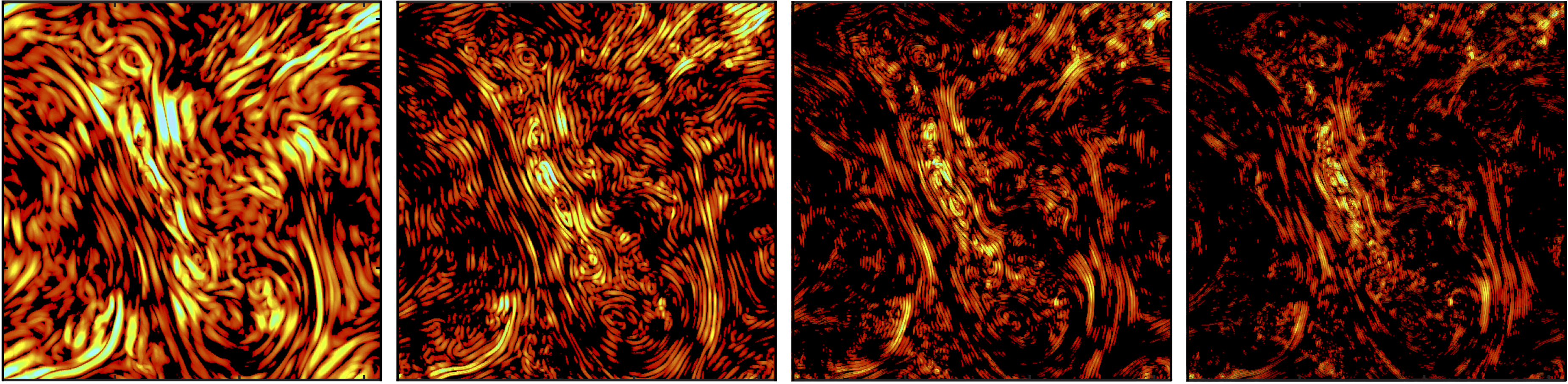
The variation of the gyrokinetic perturbed magnetic field along the unperturbed field lines
The perturbed magnetic field is shown as it varies along the unperturbed field lines (z direction). A high-pass filter is used to filter out the large scales to allow the smaller scales to become visible.
[Animations by Taran_Henk 2021, using simulations done by Dr. Daniel Told with the GENE code, data post-processed by Evgeny Gorbunov.]
Time evolution of an ideal magnetic field with a non-zero magnetic helicity
The MHD simulation is done for a viscous fluid and an ideal magnetic field (i.e. no magnetic diffusivity). As magnetic helicity is conserved in the absence of magnetic diffusivity and is non-zero in value, it will limit the lowest level the magnetic energy can decay towards (topological constraint). Since the total energy of the turbulent MHD system is not conserved due to viscosity, the energy of the turbulent flow will be completely dissipated, leaving a remanent magnetic field with a nontrivial spatial density.
[video and simulation done by Paul Bowen, as part of his undergraduate dissertation project, 2016]
Pictures
A set of pictures obtained from my work, displayed in no particular order. While the pictures are obtained through processing scientific data, and each image is related to a physical quantity or phenomena, they are selected for their overall visual appeal. A small description of each image is given, but no rigor of therms is employed.
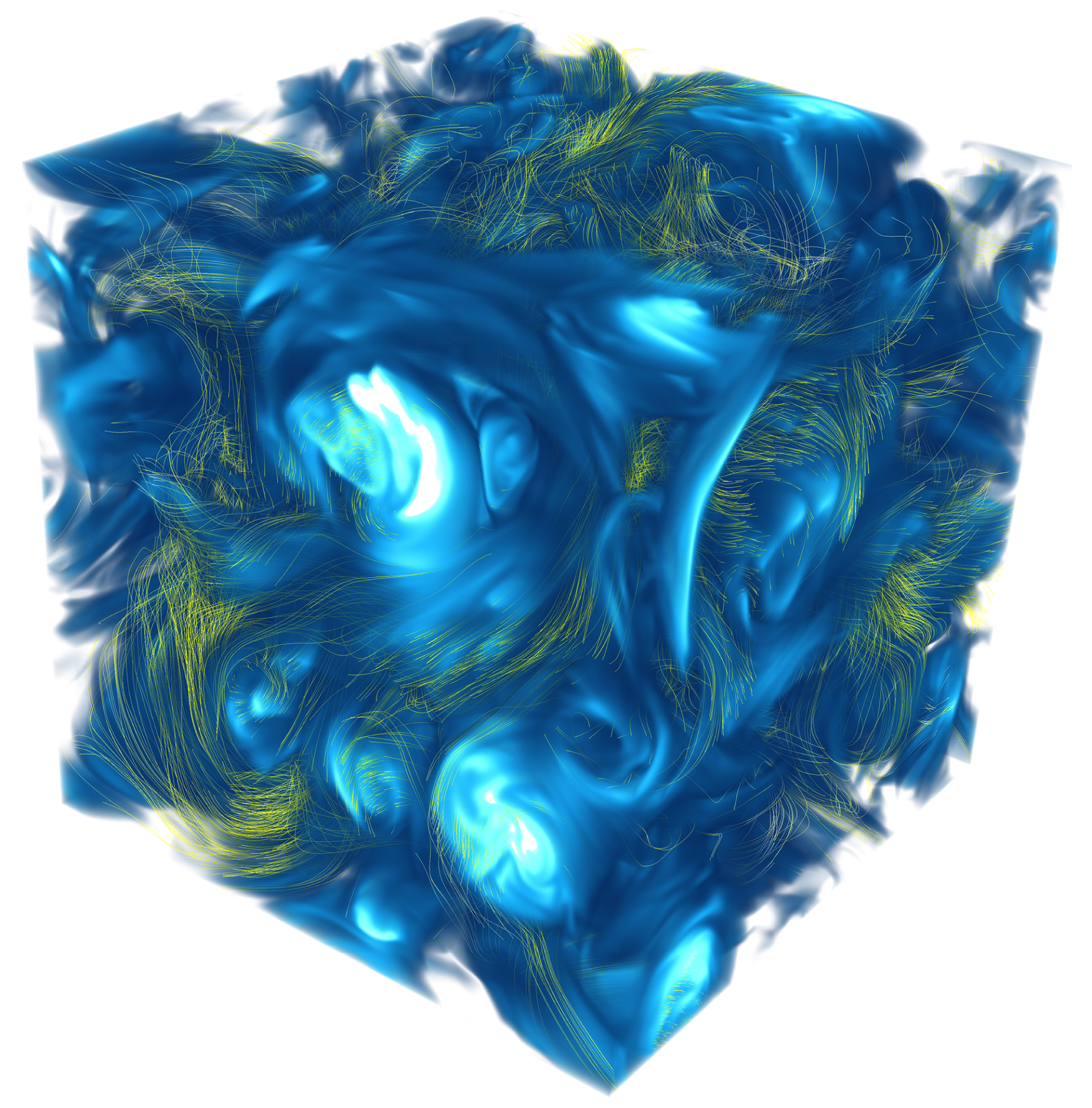
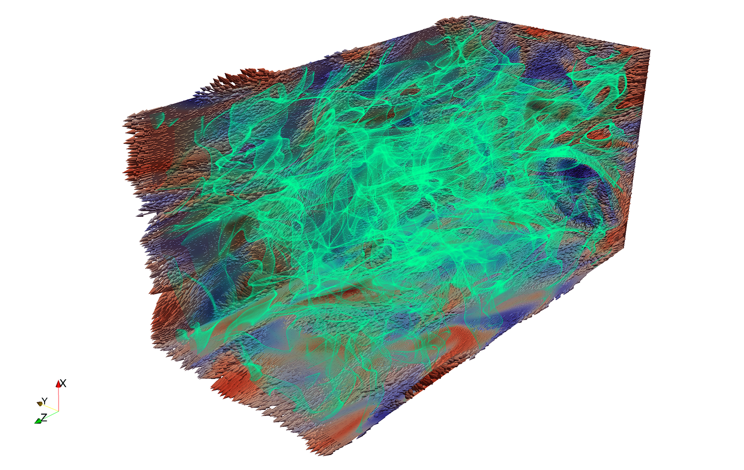
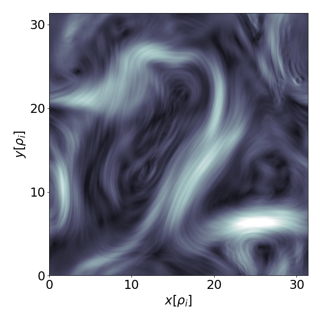
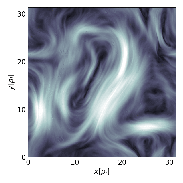
Turbulent magnetic field
Magnetic field-lines (in yellow) tracing turbulent structures denoted by the intensity of the magnetic energy (i.e. the blue cloud - lighter colors denoting larger values of the energy). As electrically charged particles move, they generate electromagnetic fields that in turn affect the trajectories of the charged particles. To a good degree, electrons can be seen as traveling along the filed-lines, while heavier ions have a tendency to bounce off magnetic structures. The picture is obtained from direct numerical simulation of magnetohydrodynamic (MHD) plasma turbulence.

Flower petals? No, just some turbulent current sheets!
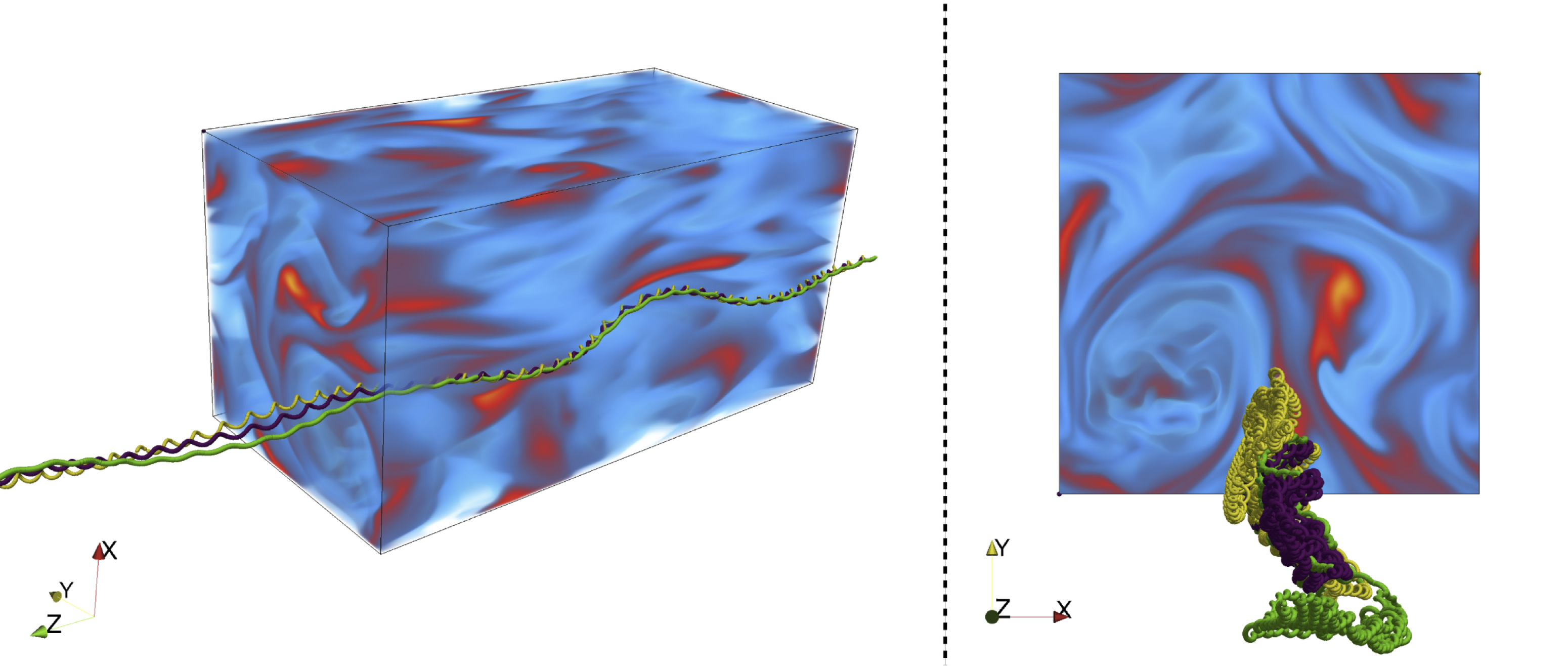
Charged particles moving inside an anisotropic magnetic field
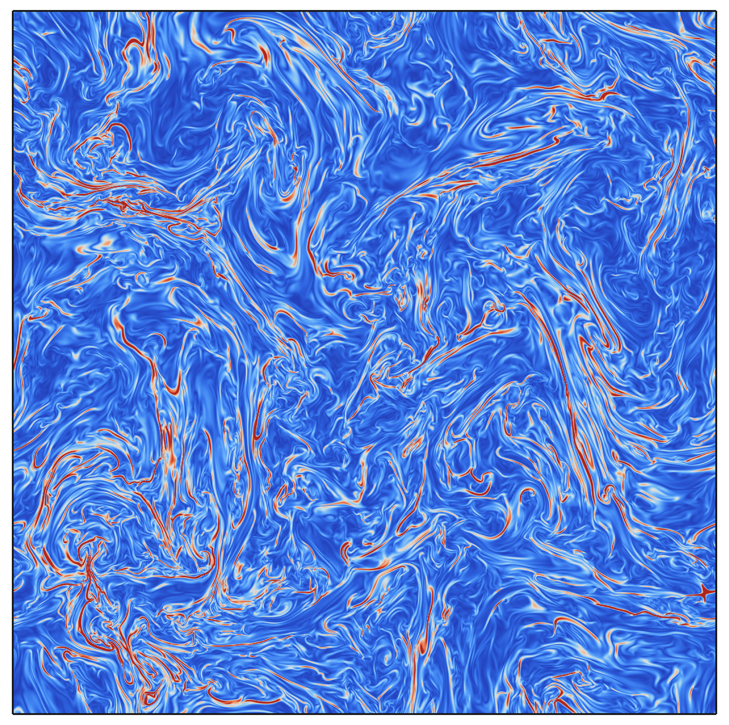
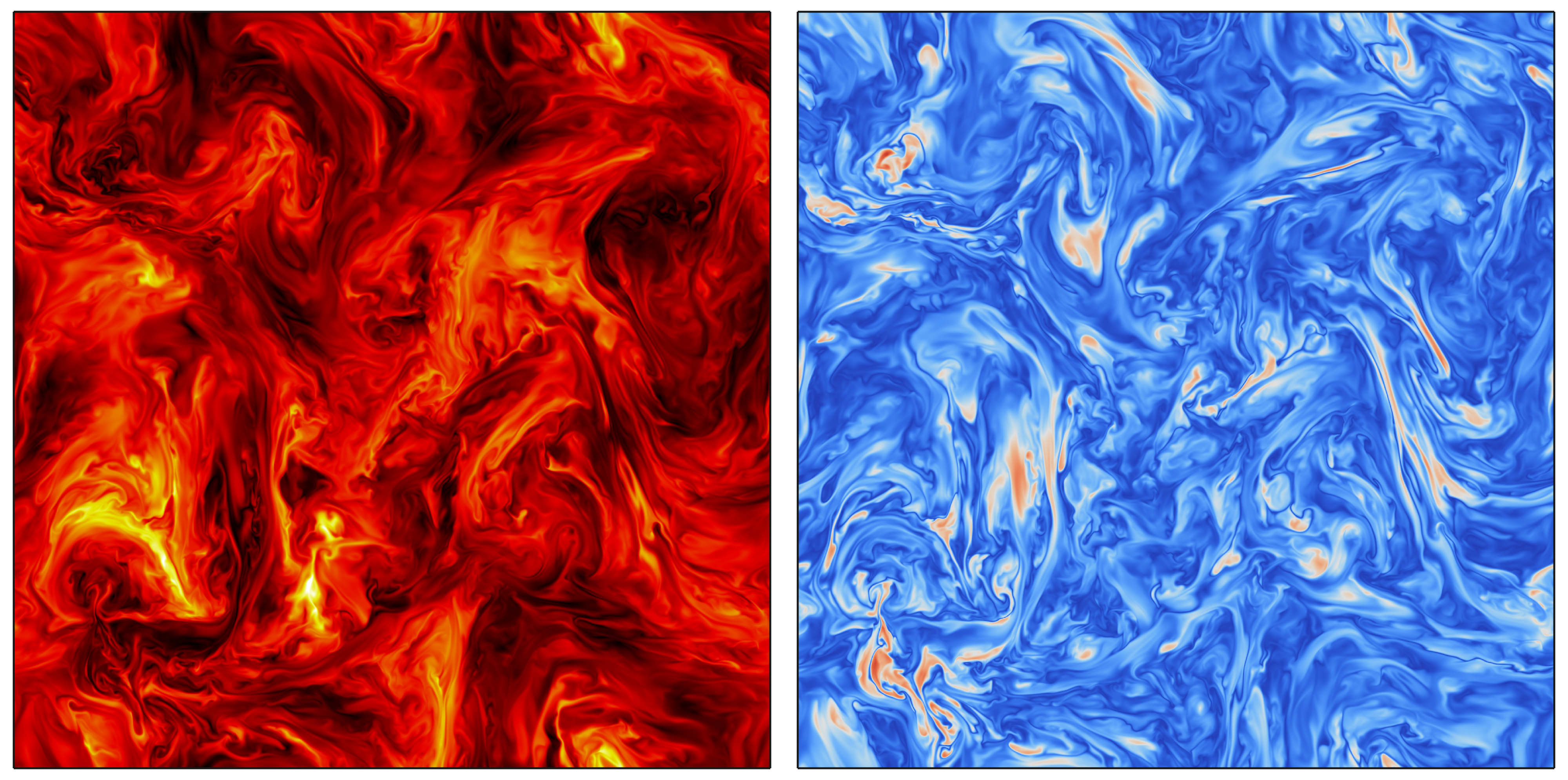
Cross-section of vortical structures in isotropic MHD turbulence
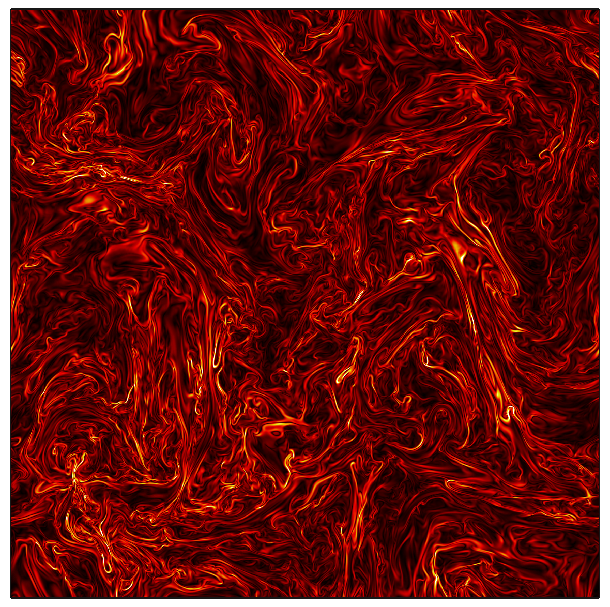
Cross-section of current structures in isotropic MHD turbulence
Fluid velocity (in red) and the self-consistent magnetic field (in blue) in MHD turbulence
A thin iso-surface of magnetic energy
The surface overlaps cuts in the three directions of the magnetic vector field, as a way to visualized turbulence in a plasma medium. As charged particles that perceive this surface as a magnetic mirror can be seen as bouncing off it and passing only through its holes, it is easy to understand why their trapped trajectories can become so intricate.
Alinement of numerical grids with density structures

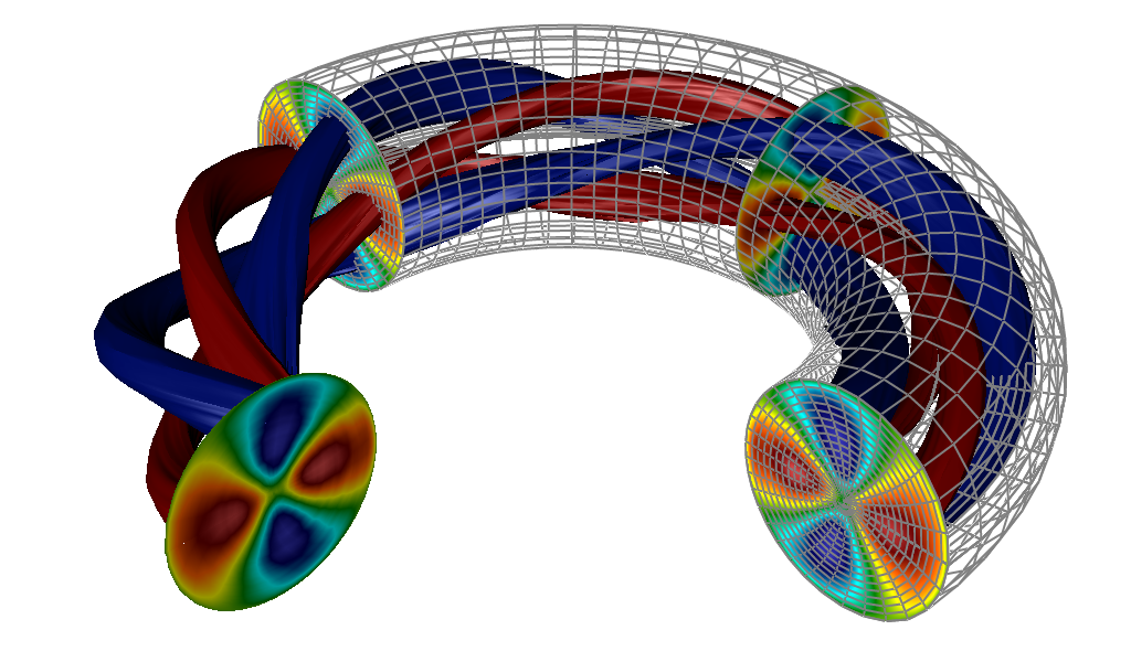
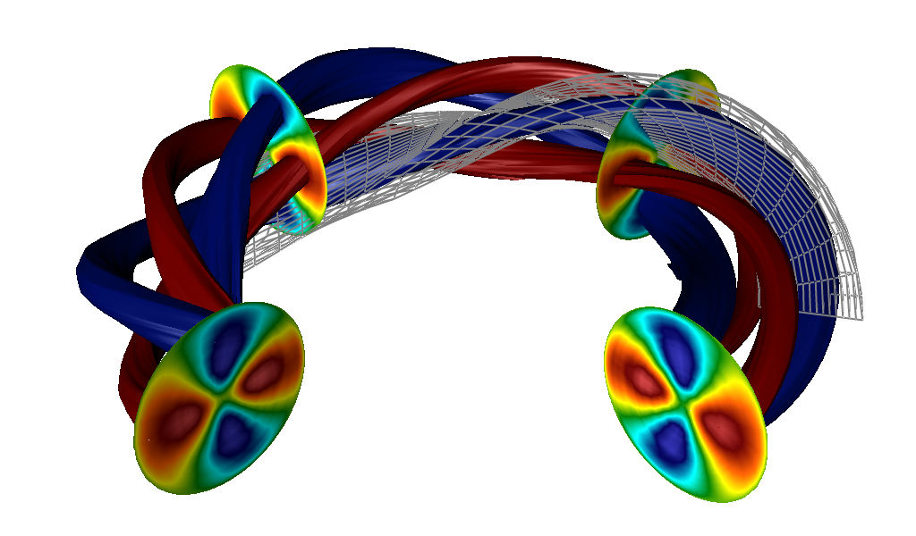
Toroidal structures in a tokamak geometry
While the figure denotes plasma density structures, these are non-physical and are obtained as a test during code development. However, non-physical does not mean non-beautiful. This image can be seen as the artistic result of scientific software.
